-
Top page
>
-
Injection molding, page 03
Page 03 (Y2025)
Structural Analysis 12 (Episode 25: Plastic gear, factor: Yf)
さて今回は JIS B1759「プラスチック円筒歯車の曲げ強さ評価方法」の中で、歯元形状係数 Yf を求めようとした時に PertPoMax を使う例を取り上げてみたいと思います。B1759 には、「歯元形状係数は、歯元すみ肉形状が標準基準ラック (JIS B1701-1) に準拠する場合 Yf = 1.0 とする。」との記載があります。そこで歯元すみ肉形状を歯車の創成曲線とした場合、および R0.375, R0.3, R0.2 とした場合をそれぞれモデリングして解析し、得られた最大発生応力から Yf を算出する試みをしてみました。
歯車は、モジュール 1.0、歯数 54、歯幅 10 mm の平歯車として、歯の部分 3 歯をモデリングして 2D サーフェイスの STEP ファイルを作成した後、PerPoMax をこれをインポートしました。この時、PrePoMax では平面ひずみでの解析を選択しました。有限要素を作成し、歯を切り取った部分を完全拘束して、ピッチ円上に相当する接点に 37.037 N を負荷しました。得られた結果の応力等高線図を下に示します。
Today, I would like to show an example of using PrePoMax to calculate the tooth root fillet factor, Yf, in JIS B1759 "Evaluation method for bending strength of plastic cylindrical gears". B1759 states that "Tooth root fillet factor shall be Yf = 1.0 when the fillet curve conforms to the standard reference rack (JIS B1701-1)". Therefore, I attempted to calculate Yf from the maximum generated stress by modeling and analyzing the cases where the root fillet curve is the gear-generating curve, where it is R0.375, R0.3, and R0.2 using PrePoMax.
The gear was a spur gear with 1.0 module, 54 number of teeth, and a facewidth of 10 mm. Just 3 teeth among the gear were modeled, the STEP file of the 2D surface was created, and then, the data were imported into PerPoMax. The plane strain analysis was selected in PrePoMax. Finite elements were created and the cut lines were fully constrained. A load of 37.037 N was applied to the node on the pitch circle. The obtained results were shown below in the contour plots.


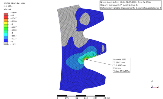
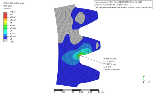
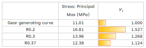
なお、解析の種類は幾何非線形を加味した静解析として、材料は PrePoMax のデータベースから POM を選択しました。以上結果を元に Yf を算出すると、左表のようになりました。ただしこれは Yf の求め方の一つの例ですので、あくまで私個人が PrePoMax の使い方の習得を目的としたものであることをご理解ください。加えてYfの算出には歯数を様々に変えたケースが必要ですので、今回はモジュール 1.0 の場合の例ということになります。
The type of analysis was static analysis with consideration of geometric nonlinearity, and POM was selected as the material from the PrePoMax database. When Yf values were calculated based on the above results, they are shown in the table on the left. However, please understand that this is just one example of how to calculate Yf and is intended only for personal learning about how to use PrePoMax. In addition, the calculation of Yf requires a case in which the number of teeth is varied; however, this is an example for module 1.0.
Structural Analysis 13 (Episode 26: Friction coefficient)
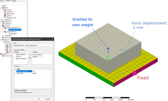
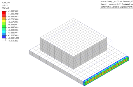
今回の解析は、材質が金属 (S185 : PrePoMax の材料データベースの値をそのまま使用) の板の上に、同じく S185 のブロックを置き、板の一端を固定したうえでブロックの端を5 mm 変位させた時の拘束点の生じる最大反力を出力することとしました。この時、解析において、接触面の Friction Coefficient を 0.1, 0.2, 0.3, 0.4 と変化させた時に、上述の反力がどのように変化するかを確認しました。PrePoMax における Friction Coefficient はおそらく摩擦係数的なものを表現するために用いられるものと思われますが、この値が反力にどのように影響を及ぼすでしょうか? 作成した有限要素モデルと解析条件の設定を図に示しています。
In this analysis, an S185 (S185: the value in the PrePoMax material database was used as is) steel block was placed on a plate made of the same material, one end of the plate was fixed, and the maximum reaction force generated at the constraint point when the end of the block was force displaced 5 mm was output. In this analysis, I confirmed how the reaction force described above would change when the "Friction Coefficient" at the contact surface was changed to 0.1, 0.2, 0.3, and 0.4. The "Friction coefficient" in PreProMax is probably used to express something like the "Coefficient of Friction", but how does this value affect the reaction force? The created finite element model and analysis conditions are shown here in picture.
結果として、Friction coefficient の値を 0.3 としたときの X 軸方向の反力コンター図を示します。また、それを変化させて、最大反力をグラフ化して表示します。
The reaction force contour plot in the X-axis direction for a friction coefficient of 0.3 is shown. In addition, by changing the values, the outputted maximum reaction forces are graphed and shown here.
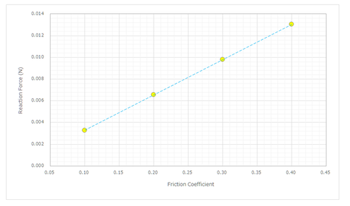
以上の結果から、"Friction coefficient" の値を変えると、拘束点に生じる反力は直線的に変化するとこがわかりました。
From the above results, it can be seen that when the "Friction coefficient" value is changed, the reaction force generated at the constraint point changes linearly.
Structural Analysis 14 (Episode 27: Bias of rotating part)
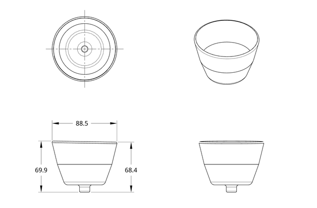
円筒形状で、さらに底部に同芯の円筒をもつ物体を、回転させた時に発生する応力と変形をシミュレーションしてみます。使用した形状は、図に示すようにコップのような形をしていますが、底部には円筒部部を有します。肉厚は 2.5 mm です。高さを見ると、左右で違いがあり、これによって回転した時に重心にズレが生じます。
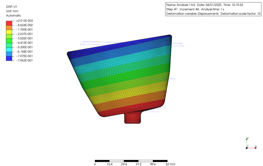
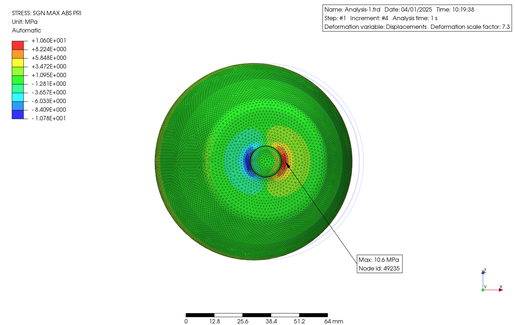
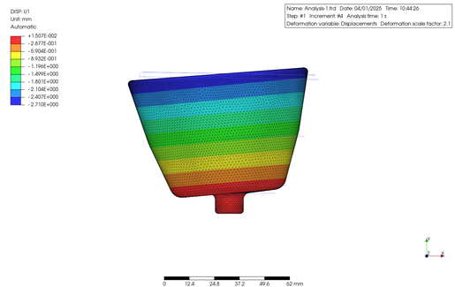
この物体の材料を ABS 樹脂として、その底円筒部の外周に沿って 800 rad/sec で回転させてみました。この時 ABS の特性は PrePoMax のデータベースをそのまま用いました。その結果を下に示します。表示は U1 軸 (X 軸) 方向の変位と最大主応力の等高線図になります。
Let me simulate the stress and deformation when a cylindrical object with a concentric cylinder at the bottom is rotated. The shape used is like a cup, as shown in the figure, but it has a cylindrical part at the bottom. The wall thickness was 2.5 mm. Looking at the height, there is a difference between the left and right sides, which causes a shift in the center of gravity when rotated.
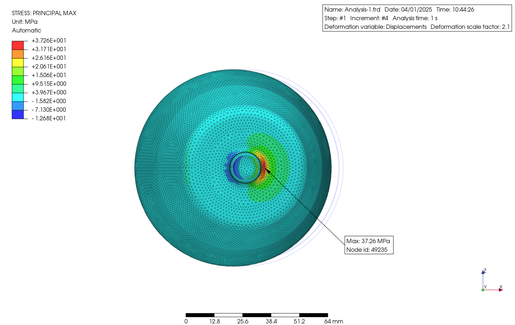
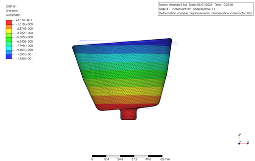
The part was made of ABS resin and rotated at 800 rad/s along the bottom cylindrical portion. The properties of ABS were extracted directly from the PrePoMax database. The results are as follows. The figure shows a contour plot of the displacement along the U1 axis (X-axis) and the maximum principal stress.
さらに、仮に上記の材料の密度が 2 倍、3 倍だったとして、すなわち上記の解析から密度の値のみをそれらの値に変更した解析を行ってみると、以下の結果が得られました。
Furthermore, if I were to hypothetically double or triple the density of the above materials, i.e., change only the density values from the above analysis to those values, I obtained the following results from those simulations.
|
U1 Max. Displacement |
Pri. Stress, Max. |
| ABS |
0.8 mm |
10.6 MPa |
| Density x2 |
2.7 mm |
37.3 MPa |
| Density x3 |
11.9 mm |
168 MPa |
これは、かなり影響していますね。密度を 3 倍にした結果なんかは、部品は破壊するようなレベルですね。
運動の際は、体重が重たい人ほど準備運動をして足首などの柔軟性を確保すこことが如何に大切なのか、良く分かりました。気をつけたいと思います。
This has a significant effect. If you triple the density, the parts would be destroyed.
Now I understand how important it is for heavier people to do warm-up exercises to ensure flexibility in the ankles and other parts of their bodies when exercising. I will be more careful!
Structural Analysis 15 (Episode 28: Nonlinear Analysis )
非線形解析というと、幾何学的非線形や材料非線形、境界非線形が挙げられますが、今回は材料非線形を取り上げてみたいと思います。ちなみに、幾何学的非線形については、既にこのサイトで取り上げて使用しています。
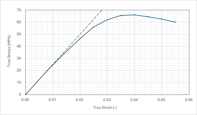
プラスチックの応力-歪曲線をみると、初期の立ち上がりこそ直線に近いものの、歪が増大するにつれて曲線になっていきます。したがって微小変形の範囲を超えて降伏点近くまでをシュミレートするためには、幾何学的非線形および材料非線形での解析が必要になります。
Nonlinear analysis can be classified into geometric nonlinearity, material nonlinearity, and boundary nonlinearity. However, this time I would like to focus on material nonlinearity. Incidentally, geometric nonlinearity has already been covered and used on this site.
If we observe the stress-strain curve of plastics, the initial slope appears as a straight line. However, as the strain increases, the curve becomes more curved. Therefore, in order to simulate large deformations beyond the range of minute deformations up to the material yield point, a geometrically nonlinear and material nonlinear analysis is required.
今回は大変形での材料の非線形性を検証するために、一本の細長い樹脂製の平板の両端を金属のブロックの上に乗せて、中央部分に一定荷重を加えた状態を PreProMax を使って有限要素解析してみましたので、その結果を以下に示します。。
In order to verify the non-linearity of the material in large deformations, I conducted Finite Element (FE) analysis using an elongated plastic flat bar supported on metal blocks at both ends, with a constant load applied to the central part using PreProMax. The results are shown below.
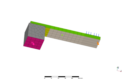
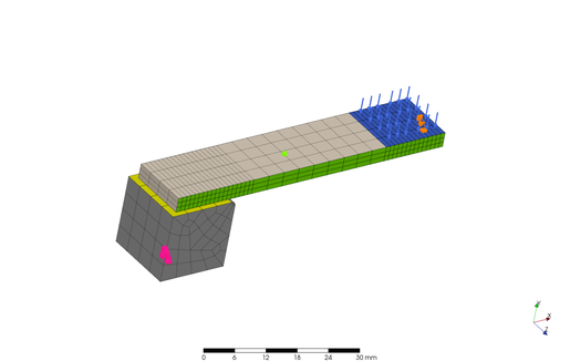
上図のようにモデのは全体の半分を要素化して、切断面には対象となるように拘束条件を設定しました。グレー色のパーツは金属ブロックであり、その下面を完全拘束してあります。平板のサイズは L: 127 mm x W: 12.7 mm x t: 3 mm です。そしてブロックとの接触面には接触を定義し、青色の中央部分の表面に 0.05 および 0.17 MPa の 2 通りの均等荷重を加えたケースをそれぞれ解析しました。なお、緑色部分には Z (横) 方向の拘束を加えています。そして、肝心の材料の特性ですが、線形解析にあたっては、縦弾性係数が 2300 MPa としましたが、材料非線形解析では、以下に示すデータを使用しました。初期の線形部分では、線形同様の縦弾性係数が得られるデータとなっています。
As shown in the above figures, half of the model was made into an element, and constraints were set so that the cut surfaces were symmetrical. The grey part is a metal block, and its bottom surface is fully constrained. The size of the bar plate is L: 127 mm x W: 12.7 mm x T: 3 mm. Contact condition was defined on the contact surface with the block, and two uniform loads of 0.05 and 0.17 MPa are applied to the blue surface at center of the part. The green surface is restrained in the Z (horizontal) direction. For the essential material properties, Young's modulus was set to 2300 MPa for the linear analysis, but the following data were used for nonlinear analysis of the material properties. In the initial linear portion, Young's modulus was set to the same value as that used in the linear analysis.
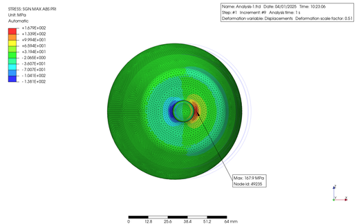
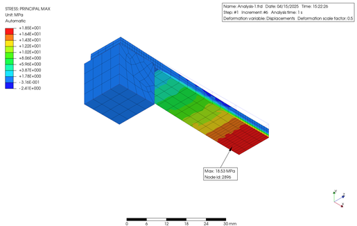
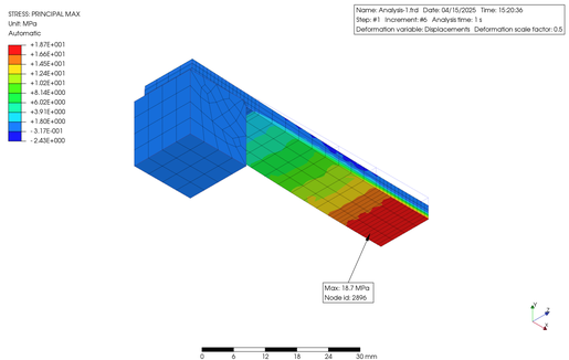
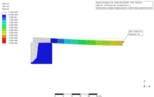
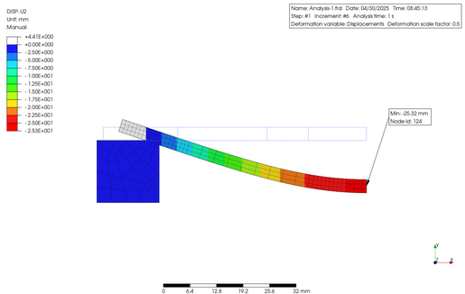
それではまず、0.05 MPa の荷重をかけたケースです。最大主応力と変位のコンター図です。材料線形と材料非線形の結果を上段・下段に表示します。いずれも幾何学的非線形で解析しています。
Let's start with the case with a load of 0.05 MPa. Here is a contour diagram of the maximum principal stress and displacement. The material linear and material nonlinear results are shown in the upper and lower rows. Both were simulated using a geometrically nonlinear approach.

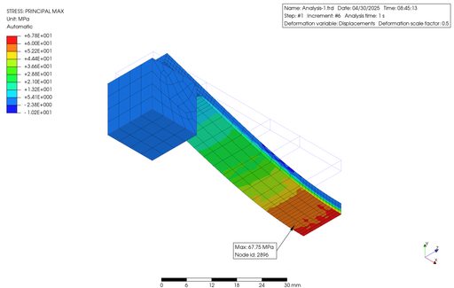
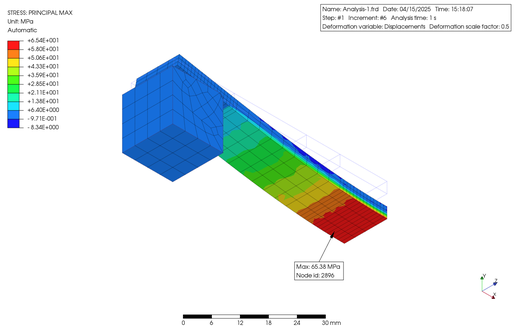
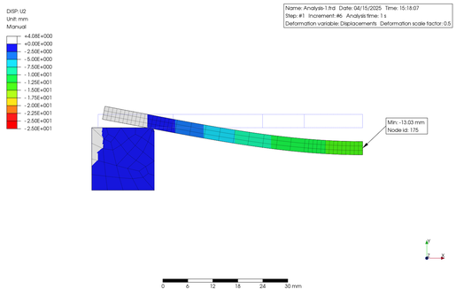
次に 0.17 MPa の荷重をかけたケースを以下に示します。上記同様に、材料線形の結果が上段で、材料非線形の結果が下段となっています。
The next case with a load of 0.17 MPa is shown below. As above, the material linear results are shown in the upper row and the material nonlinear results in the lower row.
以上の結果をまとめると、次の表のようになりました。
The above results are summarized in the following table:
|
Load: 0.05 MPa, Pri. Stress, Max. |
Load: 0.05 MPa, U2 Displacement. |
Load: 0.17 MPa, Pri. Stress, Max. |
Load: 0.17 MPa, U2 Displacement |
| Mtl Linear |
18.5 MPa |
3.7 mm |
67.8 MPa |
25.3 mm |
| Mtl Nonlinear |
18.7 MPa |
3.7 mm |
65.4 MPa |
13.0 mm |
表からわかるように。0.05 MPa 荷重下では微小変形であり、線形・非線形ともにほぼ同じ結果を示しましたが、0.17 MPa 荷重下では大変形となり、特に変位の値に大きな違いを示しました。このように、材料特性が非線形性を示すような大変形領域では、非線形データを用いた解析が必要になります。
As seen in the table, under a loading of 0.05 MPa, the deformations were small and showed nearly identical results, both linear and non-linear. However, under a loading of 0.17 MPa, the deformations were much larger, particularly the displacement values, which showed significant differences. Thus, in large deformation regions where material properties show non-linearity, analysis using non-linear data is required.
Structural Analysis 16 (Episode 29: Thermal Analysis 2)

こちらのトピックでは、射出成形関連としてスタートしたのですが、現時点では実際に成形機や金型を所有していませんので、なかなかダイレクト感のある話題をお話できていません。そこで最近ではより良い成形品をデザインするための手法として有限要素法のより構造解析を取り上げています。本来であれば、射出成形加工のシミュレーションの方がより適切とは思うのですが、その目的でフリーで使えるソフトがありません。市販のものは非常に高価格なため個人で購入する事が出来ず、現在に至っております。企業の中でたくさんの経験をしてきたのですが、開示出来ない事柄も多いため、こちらでのネタ探しに悪戦苦闘しております。もし、フリーで使える射出成形加工の解析ソフトをご存知な方は、お知らせいただけると嬉しいです。
ということで、今回は金型内の熱伝導・伝達の様子を PrePoMax を使って予測してみたいと思います。単純矩形形状のキャビティを持つ入れ子に、3種類の形状の冷却管を通して、製品部の表面温度がどのように変化していくかを見ていきたいと思います。右上に示すように、今回は 12 mm 径の直管を 4 本と、10 mm 径の直感管を 6 本、通した場合。そして、断面が四角形の冷却管を配置した場合を試してみます。因みに四角断面は底面から削り、加工部分全体を取り囲んだ O リングを介してバックプレートにより抑え込むことで実現は可能ですが、今回の解析ではバックプレートはモデル化せず、解析には用いていません。
This series has been started as an injection molding-related topic, but since I don't actually own a molding machine or mold at the moment, I could't really talk about things that have a direct feel to it. That's why recently I've been taking up structural analysis using the finite element method as a method for designing better molded products. In reality, it would be more appropriate to simulate the injection molding process, but there is no free software available for that purpose. The commercially available ones are very expensive, so individuals cannot purchase them, and that is where we are today. I have had a lot of experience in companies, but there are many things that I cannot make public, so I am struggling to find topics for this. If you know of any free injection molding analysis software, I would be grateful if you could let me know.
Therefore, this time, I want to use PrePoMax to predict heat conduction and transfer inside the mold tool. I would like to see how the cavity surface temperature changes when three different shapes of cooling channels are placed in a simple rectangular cavity insert. As shown upper right, this time I will try the scenario in which four 12 mm diameter channels and six 10 mm diameter channels are passed through is used. I will also try the case where a cooling pipe with a square cross-section. Incidentally, a square cross-section can be achieved by cutting from the bottom and holding it in place with a back plate secured with an O-ring that surrounds the entire cooling channels. However, in this analysis, the back plate was not modeled and was not used.
解析の条件は次の通りです
まず、Step 1 は、モールドベースとの接触面の温度と熱伝達率は 80°C, 1 mW/mm^2⋅°C、パーティング面の温度と境膜伝熱係数を同じく 80°C, 1 mW/mm^2⋅°C、キャビティ表面部分の温度と境膜伝熱係数は 25°C, 0.05 mW/mm^2⋅°C、そして水管の表面の温度と境膜伝熱係数を 120°C, 100 mW/mm^2⋅°C と設定しました。次に、Step 2 として、キャビティ表面部分の温度と境膜伝熱係数を 300°C, 0.1 mW/mm^2⋅°C、水管の表面の温度と境膜伝熱係数を 60°C, 100 mW/mm^2⋅°C に変化させて、それぞれの Step を 160 秒間として入れ子表面の温度変化をシミュレートしてみました。なお、入れ子の材質は PrePoMax のデータベースから S420 を選択しました。
The analysis conditions are as follows: First, in Step 1, the temperature and heat transfer coefficient of the contact plane with the mold base were set to 80°C and 1 mW/mm^2⋅°C, the temperature and film heat transfer coefficient of the parting plane were also set to 80°C and 1 mW/mm^2⋅°C, the temperature and film heat transfer coefficient of the cavity surface were set to 25°C and 0.05 mW/mm^2⋅°C, and the temperature and film heat transfer coefficient of the water channel surfaces were set to 120°C and 100 mW/mm^2⋅°C. Next, in Step 2, the temperature and film heat transfer coefficient of the cavity surface were changed to 300°C and 0.1 mW/mm^2⋅°C. At the same time, the temperature and film heat transfer coefficient of the water channel surfaces were changed to 60°C and 100 mW/mm^2⋅°C. The temperature progression of the insert was simulated in each step for 160 seconds. The material used for the insert was S420 from the PrePoMax database.
以下に示すのは、解析結果になりますが、Step 1 と Step 2 における、各々最初と最後 の Increment における入れ子表面の温度分布の等高線図になります。また、それらの下にアニメーションも添付します。
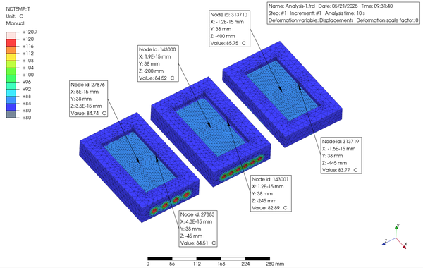
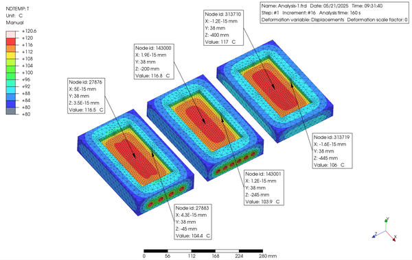
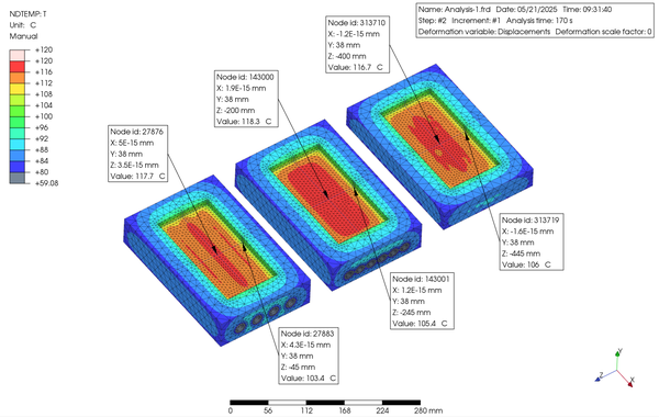
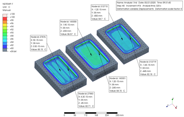
図が小さいので分かり難いかもしれませんが、これらの結果から四角断面の冷却管がより温度変化の時間が速く、またキャビティ面の温度分布が均一である傾向が見られました。したがって、特に Heat and Cool のような工法には向いているものと思われます。
Although it may be difficult to comprehend because the figure is small, these results show that a cooling pipe with a square cross section has a tendency to change temperature faster and to have a more uniform temperature distribution on the cavity surface. Therefore, it should be particularly suitable for a method such as Heat and Cool.
Optimal Molding Condition (Episode 30: Statics #01)
射出成形において、条件を決定する際に統計的な考え方を導入することは最適条件に導く良い方法の一つと思います。どんなに経験を重ねても、ただ闇雲に条件を変更していくやり方は、効率が良いとは言えません。一般的なやり方としては、まず考えられる要因の中から有意であるものを特定した後、どのような応答性があるのかを見極めた上で、最適条件を推定するような手順になるかと思います。ただし、水準の取り方や割り付け方法次第では、思うような結果が得られない場合もあるので、このあたりはやはり射出成形に対する経験が頼りになることがあるかもしれません。
In injection molding, I think that introducing statistical thinking into determining conditions is one of the best ways to achieve optimal conditions. No matter how much experience you have, simply changing conditions randomly is not an efficient method. The general approach would be to first identify the significant factors among the possible factors, then determine the types of responses, and then estimate the optimal conditions. However, depending on how the levels are chosen and how they are assigned, you may not get the results you want; therefore, you may need to rely on your experience with injection molding.
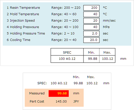
今回、右図に示すような Excel Sheet を用意しました。表中に成形条件を入力すると、仮定として、それらの条件に基づいて成形されたパーツの寸法が表示されるようになっています。もちろん擬似的なものですが、この得られた寸法値をスペック内に収められる最適条件を、統計的手法を用いて見つけていくトライをしてみたいと思います。
This time, I prepared an Excel spreadsheet shown on the right. When I enter the molding conditions in the table, the hypothetical dimensions of the part molded under those conditions are displayed. Of course, it is pseudo, but I would like to try to find the optimal conditions using statistical methods that will help achieve dimensional values within the specified specifications.
と、ここまで書いておきながらなんですが、あまりの暑さに気力が沸かないので、その結果は次回以降に持ち越しとします。あしからず・・・。
... Although I wrote this much, it was too hot, and I did not have the energy, so I will have to postpone the results until the next time. I'm sorry.
Optimal Molding Condition (Episode 31: Statics #02)
さて、前のエピソードを再開します。表を見ると、成形条件が要因として 6 種類あります。また、それぞれの設定可能な範囲が決められています。最初にするべきことは、スクリーニング、すなわち効果の少ない要因を排除して、効果があるであろう要因を見つけ出すことです。今回は、三元配置分散分析を使って上から 3 つの要因を調べた後、下の 3 要因について分析を行いました。もっと効率的な方法もあるかとは思いますが、それについては皆さんに色々試していただきたいと思います。さて、二回のスクリーニングの結果、樹脂温度、金型温度、そして保圧が有意という結果になりましたので、これら 3 つの要因で改めて三元配置分散分析を行いました。この時、水準のレベルはスクリーニングした際の区間推定結果を基に、規格値の中央付近で選定しました (下表)。
Now, let's resume from the previous episode. As you can see from the table, six types of molding conditions serve as factors. Possible ranges for each are determined. The first step is screening, which means eliminating factors that have little effect and identifying those that are likely to be effective. A three-way ANOVA was used to examine the top three factors, and the bottom three factors were analyzed. There may be more efficient ways to do this, but if you have any, I’d like you to try them out. Well, after two rounds of screening, resin temperature, mold temperature, and holding pressure were found to be significant, so I performed a three-way ANOVA on these three factors again. At this time, the level was selected near the center of the standard value, based on the interval estimation results from the screening (see the tables below).
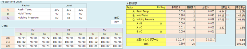
以上の分散分析の結果から区間推定を行い、そして選んだ最適条件は、樹脂温度が 220°C、金型温度が 50°C、そして保圧が 55 MPa としました。そして、これらの条件とその他の条件は範囲の中央値として 16 回のショットを繰り返し、得られた統計情報値をその下の表にしまします。これらの結果から工程能力指数 Cpk を求めると 1.37 となり、十分な能力を示しました。
From the results of the above ANOVAs, an interval was estimated, and the optimal conditions were selected as follows: resin temperature 220°C, mold temperature 50°C, and holding pressure 55 MPa. These and other conditions were set as the median values of the range, and 16 shots were repeated, and the statistical information obtained is shown in the table below. From these results, the process capability index Cpk was calculated to be 1.39, which showed sufficient capability.
| 平均値 (Mean) |
最大値 (Max.) |
最小値 (Min.)
| 標本標準偏差 (Standard Deviation, Population) |
普遍標準偏差 (Standard Deviation) |
| 99.998 mm |
100.05 mm |
99.95 mm |
0.0288 |
0.0297 |
ちなみに、エクセルで作った成形品寸法のシートですが、寸法と同時にパートコストが表示されるようにしてあります。コストを抑えつつ最適な成形条件をどのように設定したら良いかなど、いろいろな議論をしてみるのも面白いかと思います。また、分散分析は、エクセルの機能を使ったり市販のソフトを使うというよりも、ご自身でエクセルの計算式をインプットして計算ができるようにシートを作成することをお勧めします。その方が必ず良い理解に繋がりますので。
By the way, the Excel sheet that outputs part dimensions can also calculate the part cost. Various discussions, such as how to set optimal molding conditions while keeping costs low, would be interesting. For ANOVA, I recommend that you create a sheet so that you can input Excel formulas and perform calculations yourself, rather than using Excel's functions or commercially available software. This will lead to a better understanding.
Structural Analysis 17 (Episode 32: Meat Replacement)
金属に対するプラスチックの利点のひとつとして、密度が小さい事が挙げられます。しかし、強度や剛性が低いため、また射出成形での成形性考慮すると、金属と同じ肉厚では成り立たちません。そこで肉厚を増した設計が必要になってきます。今回は 内側寸法で 300 mm, 200 mm, 6 mm の A4 サイズくらいの大きさが、厚さ 0.8 mm の板金で出来ている筐体をイメージして、それをプラスチックで検討する場合を考えてみたいと思います。内容積を変えずに、外側に肉厚を増した時に、中央付近にかかる一定の圧力に対して同じ変形量となるために、どのくらいの肉厚が必要なのかを見てみることにします。
One advantage of plastic over metal is its lower density. However, due to its inferior strength and rigidity and given the moldability of injection molding, it cannot be produced in plastic at the same wall thickness as metal. This necessitates a design with increased thickness. Let us imagine a housing made of 0.8 mm sheet metal with internal dimensions of 300, 200, and 6 mm?roughly the size of an A4 sheet?and consider that it should be made of plastic. I will try to determine the wall thickness required to achieve the same amount of deformation for a given pressure applied near the center while maintaining the same internal volume as the metal.
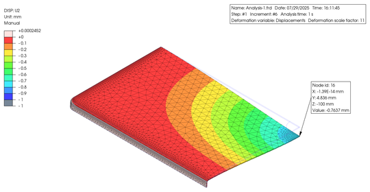
上記筐体の 1/4 有限要素モデルを 0.8 mm の肉厚で作成した後、中央部の直径 20 mm 部分に 0.1 MPa の荷重を付加した場合の垂直方向の変形量を PrePoMax を用いて静解析で求めてみました。この場合の材料は金属を想定して、ヤング率は 210 GPa、ポアソン比を 0.28、密度は 7.8 g/cm3 としました。
A 1/4 finite element model of the above housing was created with a thickness of 0.8 mm, and then a load of 0.1 MPa was applied to the central part with a diameter of 20 mm. The vertical deformation was calculated by static analysis using PrePoMax. In this case, the material is assumed to be metal, with a Young's modulus of 210 GPa, a Poisson's ratio of 0.28, and a density of 7.8 g/cm3.
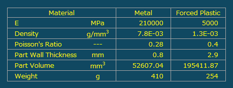
このモデルの裾部分を完全固定して解析を行うと、中央部分の高さ方向の最大変位は 0.76 mm という結果が得られました。そして、上記モデルで、強化プラスチックの特性を用いた材料を使用するとして、肉厚を外側方向に増した上で、金属と同等の変位が得られる肉厚を解析で模索すると 2.9 mm 必要であることがわかりました。 設定条件を右の表にまとめました。また、下に変位図を示します。
When analyzing this model with the bottom edges fully fixed, the maximum vertical displacement in the central section was found to be 0.76 mm. Furthermore, using the above model and assuming a material with reinforced plastic properties, analysis revealed that a wall thickness of 2.9 mm is required to achieve displacement equivalent to that of metal when increasing the wall thickness outward. The set conditions are summarized in the table on the right. A displacement diagram is also shown below.
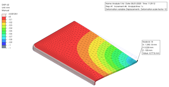
このように、薄肉の金属と同じような荷重時の変位を求めるのであれば、成形品の肉厚を増さなればなりませんが、重量低減は可能です。さらに、内側部分に干渉を避けられる空間が存在するのなら、リブを設置することによって肉厚増加を抑えられる可能性もあります。大事なことは、製品に求められる特性や機能を理解しながら、コストおよび量産性を踏まえて、バランの良い設計を模索することですね。
In this way, if we want the same displacement under load as thin-walled metal, we must increase the thickness of the molded product; however, it is possible to reduce the weight. Furthermore, if there is space inside where interference can be avoided, it may be possible to prevent an increase in thickness by adding ribs. The important thing is to understand the characteristics and functions required of the product, while also considering cost and mass productivity, and then to find a well-balanced design.
Go back to the top of this page.